Lab 2: IMU
10 minutes read •
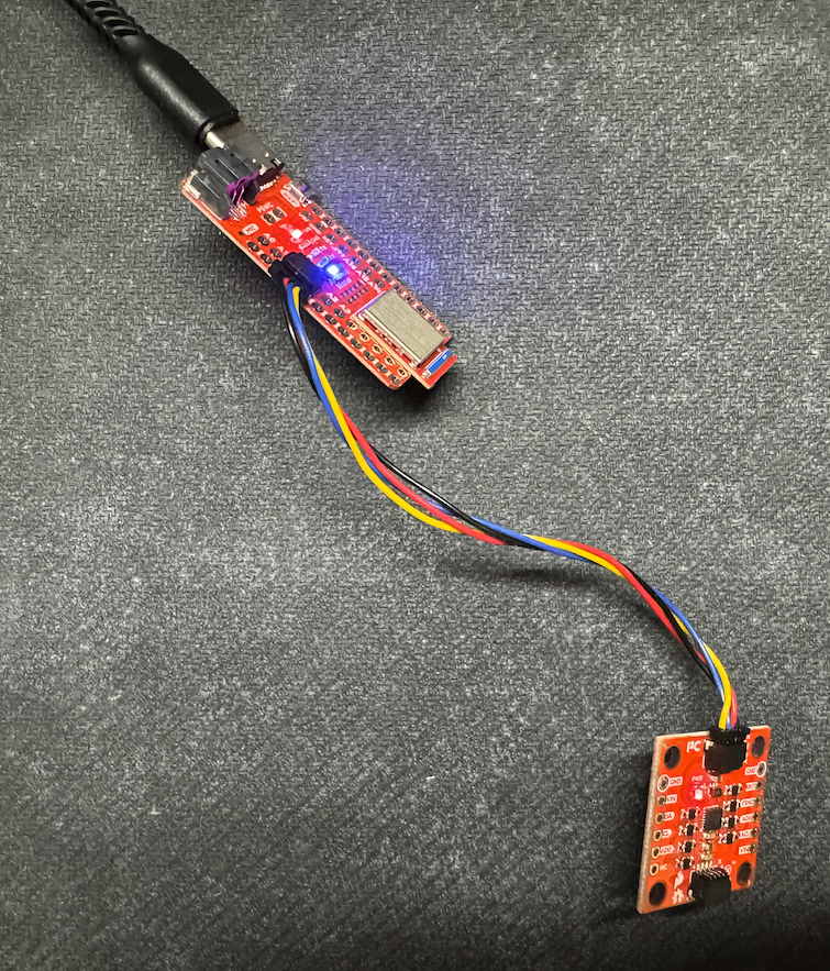
IMU Setup
AD0_VAL & Initial Data Observations
The AD0_VAL represents the last bit of the I2C address. In our case, 1 is set as the default and that shouldn’t be changed unless the ADR on the board is closed via solder and then should be set to 0.
After testing with the example code as well as the lecture 4 code, it appears that the accelerometer and gyroscope data print as expected. Three axis are printed for both sensor as well as the corresponding unit (mg for acceleration and DPF for the gyroscope). As discussed in lecture, in the data you can see accelerations and rotations being tracked but not absolute position; changes in the printed values only occur with movement. Additionally, you can see that the changing values are dependent on the axis being rotated about and the sensor being observed. When rotating around the z-axis you can see that the accelerometer data does not change, however the gyroscope does. When accelerating the board along the x-axis you can see a change in value for the accelerometer x-axis but not the gyroscope.
Accelerometer
Accelerometer Data to Pitch and Roll Conversion
pitch_a = * 180 / M_PI;
roll_a = * 180 / M_PI;
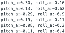
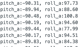
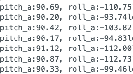
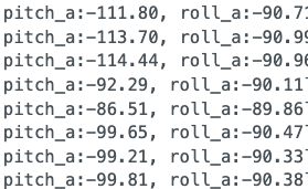
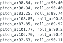
As you can see from the frozen frames, the accelerometer is very accurate with vary little variation in angle from the expected value. As a result I do not think it is nessesary to do a two-point calibration.
Data Collection and Plotting Code
The following code was used to collect the data in arrays and then use Juypter to pipe the data from the Artemis into a CSV file and graph. Note that as I added more arrays to store more data (LPF, Gyro, Complementary Filter) I simply added more columns to the csv via the notification handler. The graphs will be shown later in the lab for analysis.
Artemis Aruino Code:
case GET_ACC_READINGS:
Jupyter Code:
# Decode bytes to string & split by ";" (separating blocks)
=
# Split by "," then extract values using fast unpacking
, , =
= # Skip "P:"
= # Skip "R:"
= # Skip "T:"
# Check if file is empty, then write headers
Fourier Transform and Low Pass Filter Plotting
The raw data shows some noise in the higher frequencies however it is fairly negligable. This is due to the fact that the IMU has a low pass filter implemented already. Regardless, I will add a low pass filter
When collecting dat in the proximity of the running car, the most noise appeared to be in the range of 0 Hz and 5 Hz; I will make the cutoff at 5 Hz. The lowpass filter effects the output by limiting faster frequencies (which we are defining as noise) from being shown in the data. If the frequency chosen is too small, you will still have unwanted noise in the smaller frequency range. However, if you pick too high of a cutoff frequency you run the risk of ignoring data points that may actually be important and a correct reflection of the robot’s movement (maybe a sharp turn on a flip).
In order to apply a low pass filter I had to calculate my alpha value as 0.0876 using following equations:
$$\alpha = \frac{T}{T + RC}$$
$$ f_c = \frac{1}{2\pi RC} $$
- T = sampling rate
- $f_c$ = cutoff frequency
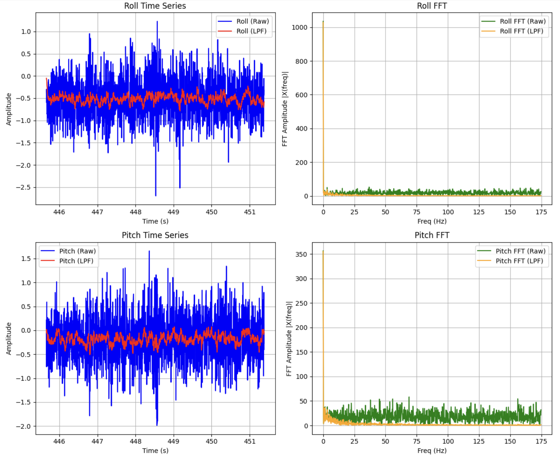
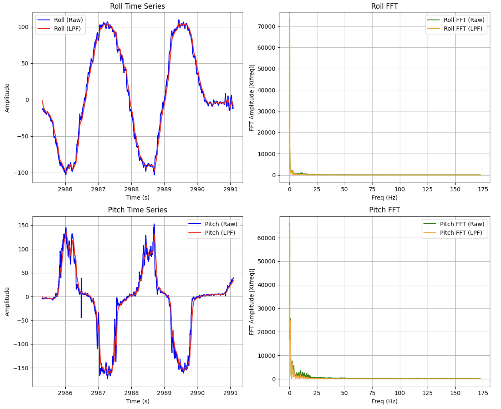
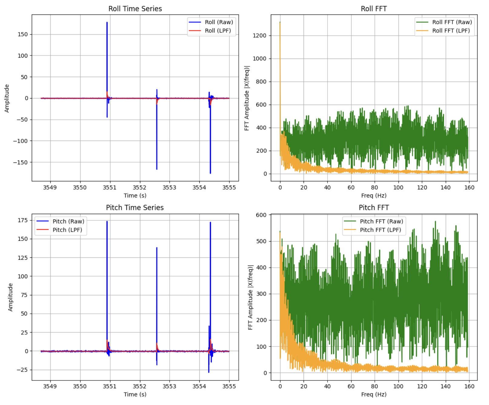
You can see that the low pass filter is successful in reducing unwanted noise in the accelerometer data. This is especially clear in the final graphic (Raw and Fourier Transform Data with Low Pass Filter - Hand Osscilations) where the LPF works to ignore the spikes in magnitude that comes from hitting the table.
Gyroscope
Equations to compute pitch, roll, and yaw angles from the gyroscope:
dt = /1000000.;
last_time = ;
pitch_g = pitch_g + myICM.*dt;
roll_g = roll_g + myICM.*dt;
yaw_g = yaw_g + myICM.*dt;
Gyroscope vs. Accelerometer Data
When first collecting the gyroscope readings I noticed that the data did not match the accelerometer data. I realized that due to the default axis of the gyroscope, the pitch and roll for the gyroscope really corresponded to the roll and pitch of the accelerometer respectively (and make the pitch negative).
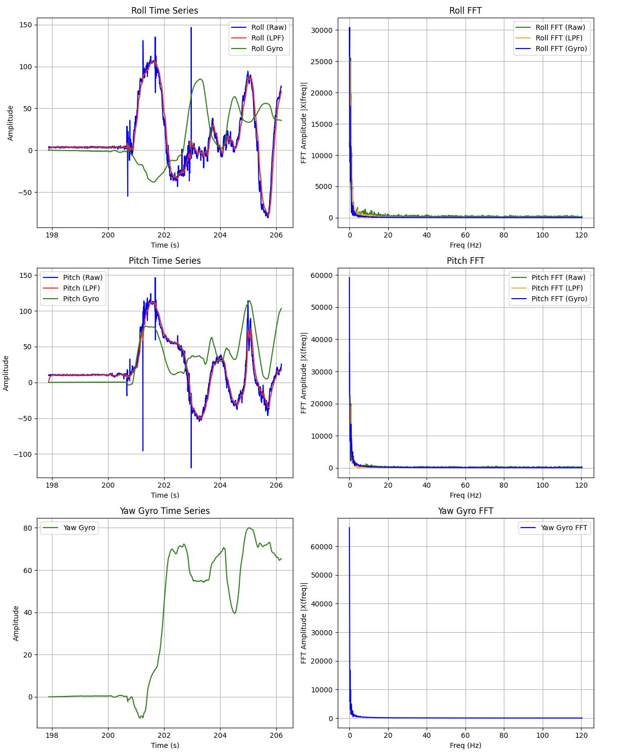
After making those changes, I noticed that there was still drift from the gyroscope over time, likely due from integrating the error in each step. However, I did find it interesting that the gyroscop provided cleaner and smoother data during quick direction changed (going from -90 to 90 degrees and back). Thus while the gyroscope alone may not be highly accurate, it is still stable.
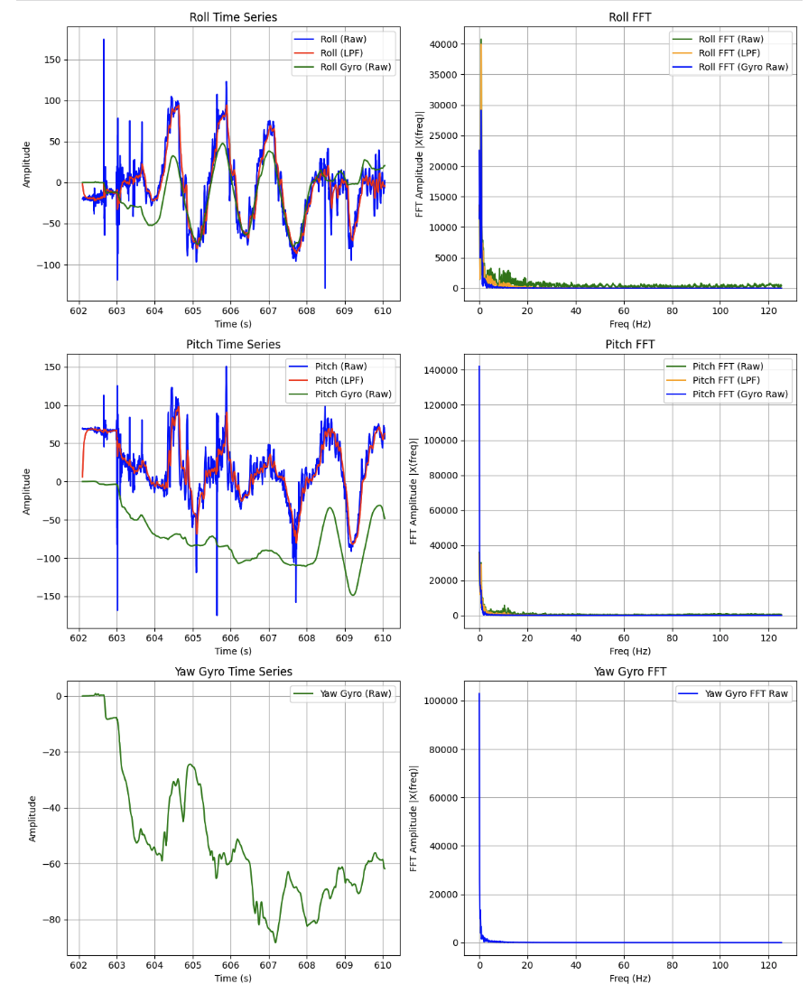
To observe the effects of changing the sampling rate, I added delays in my case GET_ACC_READINGS command code FOR loop to slow down the data collection. I noticed that a delay of 10 ms added some choppiness to the plotting without a significant increase it collection time. However, adding a 100 ms delay significantly increased the data collection time as well as the choppiness in the plot. The gyroscope, which I found was especially good at tracking quick changes of direction smoothly is now not nearly as clear. Additionally, you can see the plot jumping around for smoother IMU movements as the gaps between time intervals is increased.
Complementary Filter Implementation
The following code was used to imlpement my complementary filter:
roll_comp = * + ;
pitch_comp = * + ;
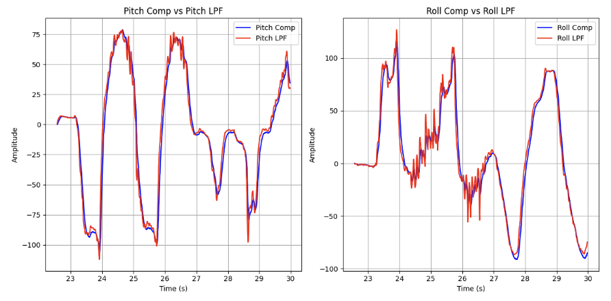
From the results you can that with an alpha value of 0.0876 the combined measurements from the accelerometer and gyroscope significantly increases stability (which comes from the gyroscope) and accuracy (from the low pass filter accelerometer).
Sampling Data
Speed Up
I took a few measures to speed up the execution time for my main loop:
- Removed the part in my code where I wait for IMU data to be ready (for example checking
(myICM.dataReady())to move through the command loop. Instead I check if data is ready in the main loop and if it is I call the functioncollectIMU()to compute the pitch, roll and yaw. After computing I add them to their respective arrays and iterate through those arrays with a different command (that does not affect the resolution as data is already collected). - Removed debugging print statments in my command to get IMU data
- I use flags to start/stop data recording
While my IMU was able to sample new values farily quickly (~ 350 Hz) after cleaning up my code, the main loop runs significantly faster than my IMU produces new data. This is evident when comparing the IMU_Count variable (which only runs when data is collected) to the Total_Loops (which counts the number of times cycled through the main). The Total_Loops is larger on the magnitude of 10-100x which means that the IMU is the holdup.
Code of main loop function:
void
collectIMU() function:
void
Jupyter code to start/stop data collection via setting a global start variable to 1 or 0 within the START_DATA_COLLECTION and START_DATA_COLLECTION commands:
import .
time.
ble.
The old case GET_ACC_READINGS command was called in Jupyter after stopping data collection to then re-popoulate the csv file with new values.
Data Storage
I decided that it would be best to have seperate arrays for storing accelerometer and gyroscope data rather than one large one. This was partially because I decided that it would be easier to organize and parse through the data using different arrays to compartmentalize the data before sending them over bluetooth. I also found it easier to create a CSV from the seperate arrays in Jupyter.
Each of these arrays contain floats as the gyroscope and acceleration naturally output decimal values. With a double data type being twice the size of a float (64 vs 32 bits), I decided that a float was the best data type for these sensor arrays.
I have a total of 10 floats arrays for a total of 40 bytes at a time:
- 1 for time
- 2 for accelerometer roll and pitch
- 2 for LPF roll and pitch
- 3 for gyroscope roll, pitch, and yaw
- 2 for complementary filter data
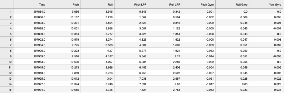
In lab 1b global variables use 30,648 bytes. This lab we added the above arrays to send IMU data. If the Artemis board has 384 kB of RAM, then 353,352 bytes of dynamic memor remain which allow us to store 353,352/40 = 8833 data points. With an average step time of 2.86 ms (shown below) we get a sample rate of 349.65 Hz. This corresponds to 25.26 seconds of IMU data collection.
5 Seconds of IMU Data
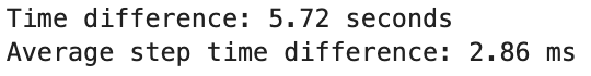
I used one of my CSV files as an example of collecting at least 5 seconds of data and sending it over bluetooth. To do this I took the difference between the first time stamp and the last time stamp in my proximityFinal.csv file:
import pandas as # Load the CSV file
df = pd.
# Get the first and last time values
first_time = df.iloc
last_time = df.iloc
# Compute the difference
time_difference = last_time - first_time
time_difference_sec = time_difference/1000
time_difference_avg = /
RC Stunts
The car is quick at direction changing and accelerating. When spinning it is able to hold its position on the ground without drifting much. Note that the car’s speed can not be changed while moving, it can only stop and change directions.
Collaboration
I collaborated extensively on this project with Jack Long and Trevor Dales. I referenced Daria’s site for code debugging in my complementary filter as well as visually understanding how to effectively display my plots. ChatGPT was heavily used to write plotting code for the Raw, FFT and LPF data. It also helped me write my FFT function as the provided link had some syntax error and missing pictures.